Analysis Frequentist Approach

This tutorial shows how to perform post-test analysis of an A/B test experiment with two variants, so called control and treatment groups, using frequentist statistics. It handles both the case of means comparison and conversions comparison with closed-form-solutions. It assumes that sample data are normally distributed.

Let’s import first the tools needed.

import numpy as np
from abexp.core.analysis_frequentist import FrequentistAnalyzer
from abexp.visualization.analysis_plots import AnalysisPlot

Compare means

Here we want to compare the mean of the control group versus the mean of the treatment group given the sample observations.

# Define the analyzer
analyzer = FrequentistAnalyzer()

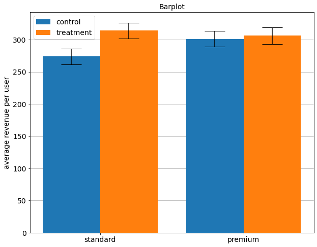
We will compare the average revenue per user of the control group versus the treatment group, making separate analysis for standard and premium users.

# Revenue for standard users
np.random.seed(42)
revenueS_contr = np.random.normal(270, 200, 1000)
revenueS_treat = np.random.normal(300, 200, 1000)

# Revenue for premium users
revenueP_contr = np.random.normal(300, 200, 1000)
revenueP_treat = np.random.normal(310, 200, 1000)

pval_S, ciS_contr, ciS_treat =  analyzer.compare_mean_obs(obs_contr=revenueS_contr,
                                                          obs_treat=revenueS_treat,
                                                          alpha=0.05)

pval_P, ciP_contr, ciP_treat =  analyzer.compare_mean_obs(obs_contr=revenueP_contr,
                                                          obs_treat=revenueP_treat,
                                                          alpha=0.05)

print('Standard users: p-value = {:.6f}'.format(pval_S))
print('Premium  users: p-value = {:.6f}'.format(pval_P))

Standard users: p-value = 0.000005
Premium  users: p-value = 0.571544

If p-value \(\leq\)0.05 the test result is statistically significant. There is a significative difference between control and treatment groups.

Otherwise if p-value \(>\) 0.05 the test result is not statistically significant. There is not a statistical significant difference between control and treatment groups.

# Computer groups mean
meanS_contr = np.mean(revenueS_contr)
meanS_treat = np.mean(revenueS_treat)
meanP_contr = np.mean(revenueP_contr)
meanP_treat = np.mean(revenueP_treat)

Display test results in barplots.

# Define height of the control group bars
bars_contr = [meanS_contr, meanP_contr]

# Define height of the treatment group bars
bars_treat = [meanS_treat, meanP_treat]

# Define upper and lower limit of the error bars for the control group
ci_contr = [[ciS_contr[0], ciP_contr[0]],  #  2.5 percetiles
            [ciS_contr[1], ciP_contr[1]]]  # 97.5 percentiles

# Define upper and lower limit of the error bars for the treatment group
ci_treat = [[ciS_treat[0], ciP_treat[0]],  #  2.5 percetiles
            [ciS_treat[1], ciP_treat[1]]]  # 97.5 percentiles

bars = [bars_contr, bars_treat]
ci = [ci_contr, ci_treat]

fig = AnalysisPlot.barplot(bars, ci, title='Barplot',
                           ylabel='average revenue per user',
                           xlabel=['standard', 'premium'],
                           groupslabel=['control', 'treatment'])

Compare conversions

Here we want to compare the number of user that made a purchase in the control group versus the treatment group.

# Number of users that made a purchase
purchase_contr = 400
purchase_treat = 470

# Total number of users
total_usr_treat = 5000
total_usr_contr = 5000

p_val, ci_contr, ci_treat = analyzer.compare_conv_stats(conv_contr=purchase_contr,
                                                        conv_treat=purchase_treat,
                                                        nobs_contr=total_usr_treat,
                                                        nobs_treat=total_usr_contr)

print('p-value = {:.6f}'.format(p_val))

p-value = 0.013002

In this case p-value \(\leq\)0.05, the test result is statistically significant. There is a significative difference between control and treatment groups. The treatment applied on the test group was successful.