Analysis Bootstrap

This tutorial shows how to perform analysis after A/B test experiments using bootstrapping. This technique makes inference about a certain estimate (e.g. sample mean) for a certain population parameter (e.g. population mean) by resampling with replacement from the observed dataset. It does not make any assumption on the samples distribution.

Let’s import first the tools needed.

import numpy as np
import pandas as pd
from abexp.core.analysis_frequentist import FrequentistAnalyzer
from abexp.visualization.analysis_plots import AnalysisPlot

Simple bootstrap

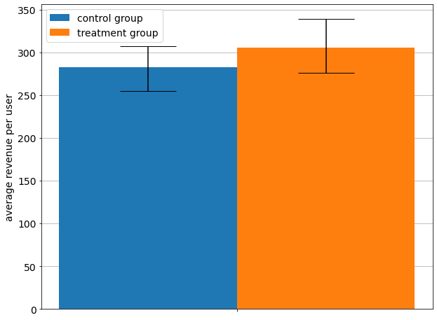
Here we want to compare a specific metrics of the control group versus the treatment group (e.g. average revenue per user). We will perform bootstrapping on the kpi metrics (revenue) of each group.

# Generate random data for revenue control group
revenue_contr = np.random.randint(low=50, high=500, size=100)

# Generate random data for revenue treatment group
revenue_treat = np.random.randint(low=50, high=600, size=100)

# Define the analyzer
analyzer = FrequentistAnalyzer()

# Define the aggregation function that will be applied on the sample
aggregation_func = np.mean

# other possibles aggregation functions might be:
#  - standard deviation = np.std,
#  - sum                = np.sum
#  - median             = lambda x: np.median(x, axis=0)

Bootstrapping will generate a sequence of N values (where N is the number of repetitions). The bootstrap function returns a table with the median, 2.5 percentile and 97.5 percentile of this sequence.

# Perform bootstrapping on the control group
stats_contr = analyzer.bootstrap(revenue_contr, func=aggregation_func, rep=500)
stats_contr

	median	2.5 percentile	97.5 percentile
	282.475	255.092	307.1285

# Perform bootstrapping on the treatment group
stats_treat = analyzer.bootstrap(revenue_treat, func=aggregation_func, rep=500)
stats_treat

	median	2.5 percentile	97.5 percentile
	305.5	276.192	339.1205

# Define heights of the bars
bars = [stats_contr['median'], stats_treat['median']]

# Compute the error between median and percentiles
ci_contr = [stats_contr['2.5 percentile'],
            stats_contr['97.5 percentile']]

ci_treat = [stats_treat['2.5 percentile'],
            stats_treat['97.5 percentile']]

# Plot results with confidence interval
fig = AnalysisPlot.barplot(bars, [ci_contr, ci_treat],
                           groupslabel=['control group', 'treatment group'],
                           ylabel='average revenue per user', xlabel='')

In the barplot above we see that there is no difference between empirical means because the confidence intervals overlap.

Time series bootstrap

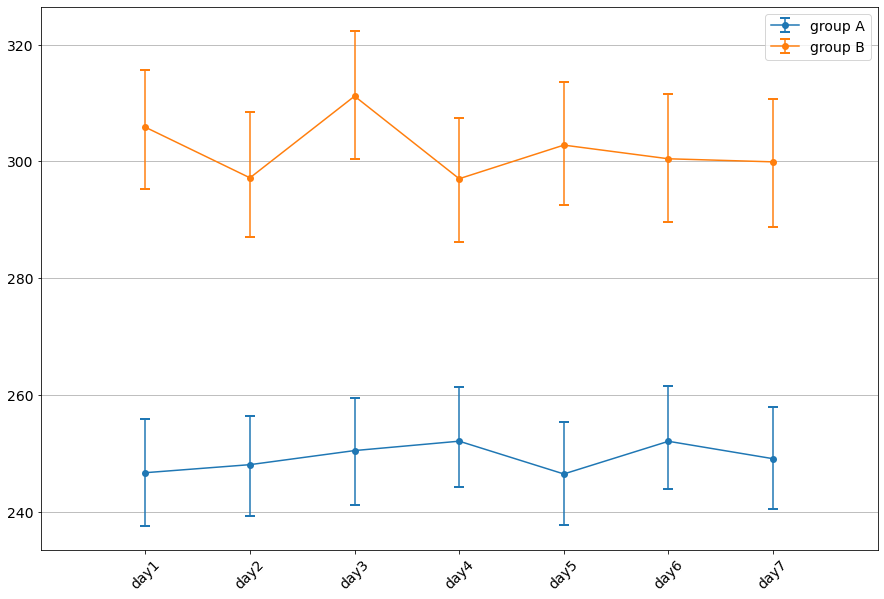
Here we want to compare a specific metrics of the control group versus the treatment group (e.g. average revenue per user) across time. We will perform bootstrapping on the kpi metrics (revenue) of each group per each day. Note that the bootstrap function maintains the correlation across days.

# Generate random data for revenue control group
revenue_contr_ts = pd.DataFrame({'day1': np.random.randint(low=1, high=500, size=1000),
                                 'day2': np.random.randint(low=1, high=500, size=1000),
                                 'day3': np.random.randint(low=1, high=500, size=1000),
                                 'day4': np.random.randint(low=1, high=500, size=1000),
                                 'day5': np.random.randint(low=1, high=500, size=1000),
                                 'day6': np.random.randint(low=1, high=500, size=1000),
                                 'day7': np.random.randint(low=1, high=500, size=1000)})

# Generate random data for revenue treatment group
revenue_treat_ts = pd.DataFrame({'day1': np.random.randint(low=1, high=600, size=1000),
                                 'day2': np.random.randint(low=1, high=600, size=1000),
                                 'day3': np.random.randint(low=1, high=600, size=1000),
                                 'day4': np.random.randint(low=1, high=600, size=1000),
                                 'day5': np.random.randint(low=1, high=600, size=1000),
                                 'day6': np.random.randint(low=1, high=600, size=1000),
                                 'day7': np.random.randint(low=1, high=600, size=1000)})

# Perform bootstrapping on the control group
stats_contr_ts = analyzer.bootstrap(revenue_contr_ts, func=aggregation_func, rep=500)
stats_contr_ts

	median	2.5 percentile	97.5 percentile
day1	246.6630	237.597475	255.912150
day2	248.0410	239.164575	256.451925
day3	250.4535	241.068275	259.431525
day4	252.0625	244.145850	261.326350
day5	246.4465	237.647800	255.376150
day6	252.0445	243.933075	261.501475
day7	249.0605	240.451950	257.918600

# Perform bootstrapping on the treatment group
stats_treat_ts = analyzer.bootstrap(revenue_treat_ts, func=aggregation_func, rep=500)
stats_treat_ts

	median	2.5 percentile	97.5 percentile
day1	305.8540	295.303525	315.689025
day2	297.1785	287.122225	308.437950
day3	311.1690	300.329400	322.258075
day4	297.0245	286.180500	307.432525
day5	302.7850	292.530300	313.642875
day6	300.4425	289.563675	311.556775
day7	299.9155	288.822375	310.642600

Plot results with confidence intervals

# Define heights of the bars
y = [stats_contr_ts['median'], stats_treat_ts['median']]

# Compute the error between median and percentiles
ci_treat_ts = [stats_treat_ts['median'] - stats_treat_ts['2.5 percentile'],
               stats_treat_ts['97.5 percentile'] - stats_treat_ts['median']]
ci_contr_ts = [stats_contr_ts['median'] - stats_contr_ts['2.5 percentile'],
               stats_contr_ts['97.5 percentile'] - stats_contr_ts['median']]

fig = AnalysisPlot.timeseries_plot(y, [ci_contr_ts, ci_treat_ts])